Chapter 6 Multivariate Strategies
6.1 Summary

We live in a complex world and many of the variables you investigate are impacted by, or associated with, more than one variable. Therefore, it’s important that when visualising data, you can use methods for visualising complex multivariate relationships. In fact, it is often through data visualisation that the impact of many variables working in combination can be perceived. However, as data complexity increases you will face a greater challenge to ensure your designs remain accessible and intuitive. In the chapter that follows you will explore various strategies for visualising multivariate data. The chapter will contain many datasets and case studies exploring the use of ggplot2, as well as some purpose-built methods and tools, for multivariate data visualisation.
6.1.1 Learning Objectives
The learning objectives associated with this chapter are:
- List and explain the four most common strategies for visualising multivariate data, which includes mapping additional aesthetics, faceting, using purpose-built multivariate visualisations and animation.
- Demonstrate the ability to design data visualisations that incorporate a range of variables of different types to tell focused multivariate data stories.
- Use
ggplot2and other purpose-built data visualisation tools to create and customise common multivariate data visualisations. - Use
Rto wrangle data into the necessary data structures required to appropriately visualise multivariate data. - Critically appraise common multivariate data visualisations and exercise judicious choice when selecting an appropriate multivariate display of the data.
6.2 Multivariate Thinking
The first time you learnt statistics, you probably focused on statistical models that had no more than two variables, e.g. simple regression and correlation, Chi-square test of association, t-tests, and one-way ANOVA. The introductory course presents a simplified, bivariate view of the world. This is done for a pedagogical reason. You need to master the basics of statistics before you move onto multivariate statistics. The real world is not bivariate. You must develop a multivariate mindset by always considering how combinations of variables might help explain or interact with your variable of interest. Multivariate data visualisation strategies can help you to discover and communicate multivariate relationships. However, there is a limit to the number of dimensions that the human brain can reason with. For that reason, multivariate data visualisations require careful design.

To start the chapter, let’s consider an example that highlights the importance of multivariate thinking. Do children and adolescent smokers tend to have poorer lung function than non-smokers as measured by forced expiratory volume (FEV). FEV is measured by spirometry as the volume of air in litres expelled in a single breath within a given time (typically 1 second). The FEV.csv dataset contains the FEV, smoking status, age, height and sex of a sample of 654 children and adolescents aged between 3 and 19 (Mean = 9.93, SD = 2.95). Sample consisted of 589 nonsmokers (90%) and 65 smokers (10%).
In the bivariate world, you would start with a side-by-side box plot with mean and error bars (95% CI)
FEV = read.csv("data/FEV.csv")
p1 <- ggplot(data = FEV, aes(x = smoking, y = FEV))
p1 + geom_boxplot() + stat_summary(fun.y = "mean", geom = "point",
                                   colour = "red") +
  stat_summary(fun.data = "mean_cl_boot", colour = "red",
               geom = "errorbar", width = .2)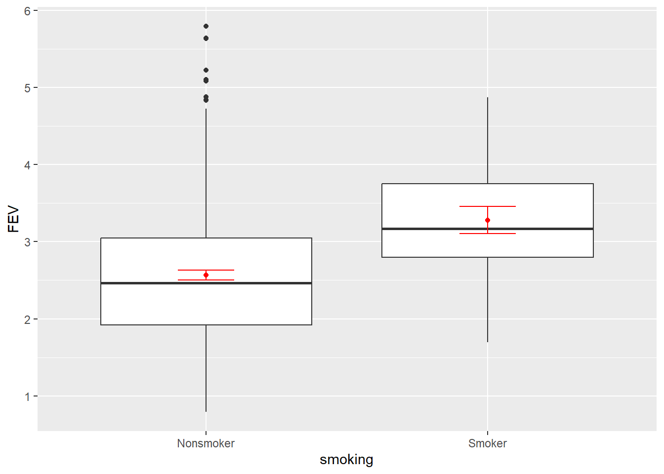
Huh? Smokers tend to have higher FEV than non-smokers. This doesn’t fit with our understanding of the negative impact of smoking. Do you stop here and publish your findings? Absolutely not. Your next step is to consider other variables that might explain what’s happening. Let’s look at all the bivariate relationships in one visualisation using the GGally package.
library(GGally)
ggpairs(FEV, columns = 1:5,axisLabels = "internal")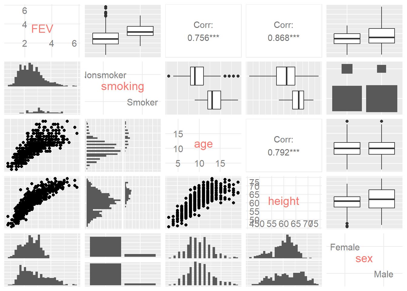
The ggpairs() function plots a matrix of bivariate data visualisations that depends on the type of variables being visualised (factor vs. numeric). You can see that when two numeric values are visualised (FEV vs. age) a scatter plot and correlation is reported. When a factor and numeric variable are visualised (smoker vs. age) a side-by-side histogram and boxplot are reported. When the two variables are factors (smoking vs. sex), faceted bar charts are shown. Looking at this matrix we can see that many of the variables are related. See if you can confirm the following:
- FEV is positively related to age and height
- Height and age a positively related.
- Smokers tend to be older and taller
Now things are starting to make sense. If FEV is related to age and height, which reflects lung growth, and smokers tend to be older and taller, then the difference in FEV might be explained solely by the lung size of the smokers. In other words, if the relationship between FEV and height (which is more strongly related to FEV, \(r = .868\) than age, \(r = .756\)) is controlled, does the difference between smokers and non-smokers hold?
p2 <- ggplot(data = FEV, aes(x = height, y = FEV, colour = smoking))
p2 + geom_point() + geom_smooth(method = "lm")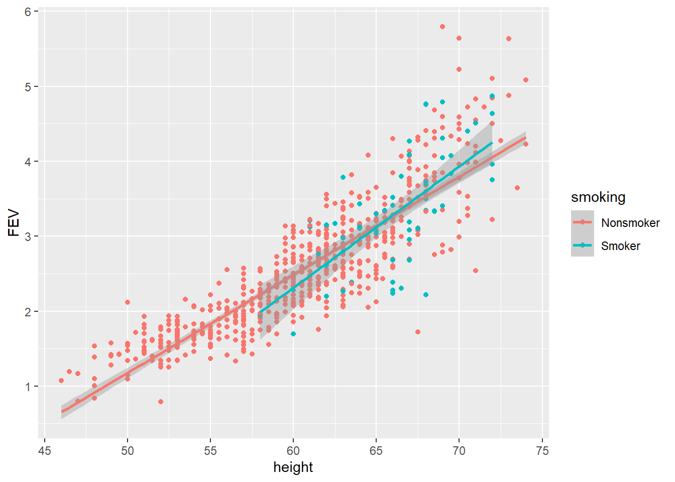
According to the scatter plot above, the smoker’s regression line is very close to the non-smokers. If the smoker’s regression line fell below and parallel to the non-smoker’s it would suggest that the mean FEV for smokers was lower. This would be an example of a main effect. If the smoker’s regression line showed a significantly different slope (e.g. flat or negative) to the non-smokers it would suggest an interaction effect. In other words, the relationship between height and FEV depends upon whether a person is a smoker or non-smoker.
This scatter plot explains the surprising finding from the boxplot. Smokers were older and therefore had bigger lungs. You should not stop there. Other variables can be explored. For example, does gender play a role? Facets make this easy to do.
p3 <- ggplot(data = FEV, aes(x = height, y = FEV, colour = smoking))
p3 + geom_point() + geom_smooth(method = "lm") + facet_grid(. ~ sex)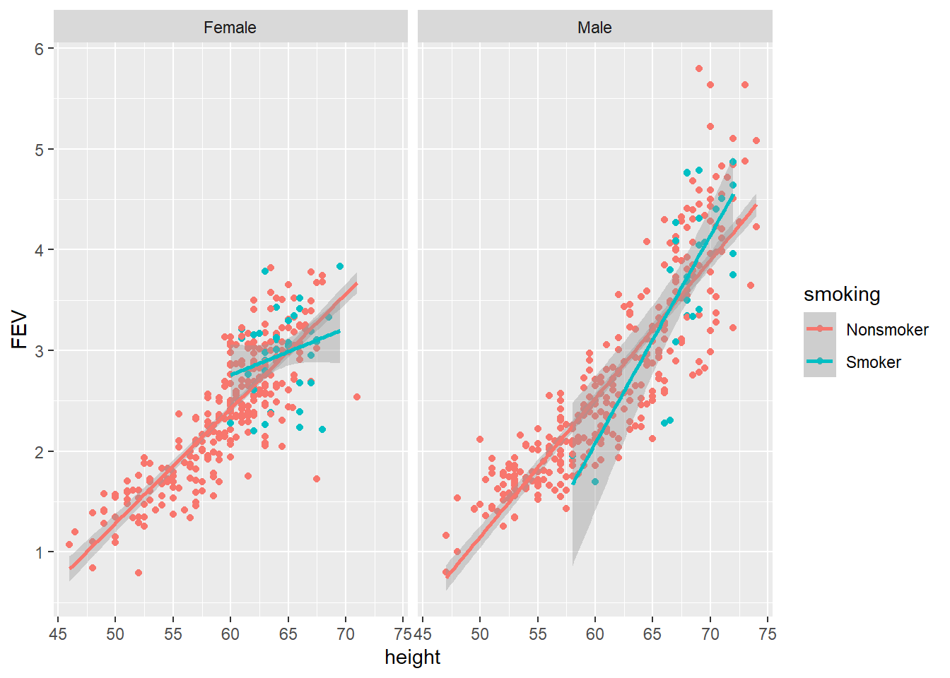
There isn’t any obvious trend, but the regression line for female smokers looks a lot different to female non-smokers. This is interesting but further data would be needed to get better estimates. How far can your go? Can you visualise all variables in one plot? That’s tricky because you have three numeric variables (FEV, height and age) and two factors (smoking and sex). You can try mapping an additional aesthetic to the plots such as alpha = age.
p3.2 <- ggplot(data = FEV,
               aes(x = height, y = FEV, colour = smoking, alpha = age))
p3.2 + geom_point() + geom_smooth(method = "lm") + facet_grid(. ~ sex)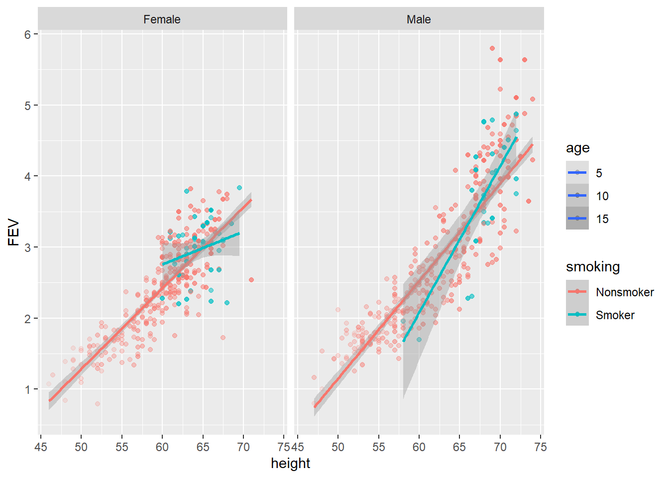
However, alpha, like a colour aesthetic, lacks visual accuracy and the viewer will find it hard to discern.
Another strategy would be to convert age to a binary variable such as children (< 10) and adolescents (10 - 19). This would allow you to use a double facet and squeeze one more variable into the plot.
FEV$age_cat <- ifelse(FEV$age < 10, "Children", "Adolescent")
p3.3 <- ggplot(data = FEV,
               aes(x = height, y = FEV, colour = smoking))
p3.3 + geom_point() + geom_smooth(method = "lm") + facet_grid(age_cat ~ sex)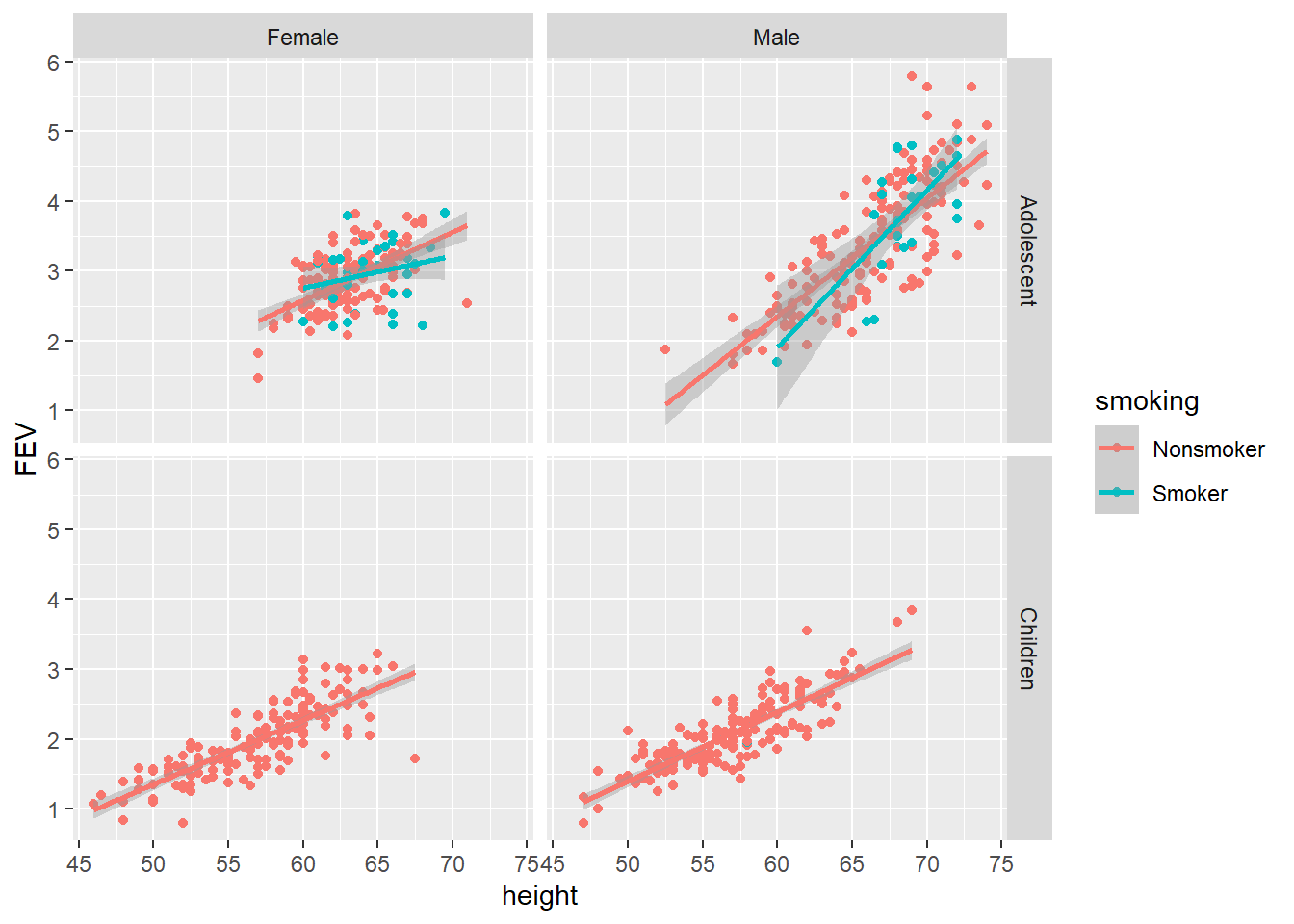
This is the maximum number of variables that should be included in any single data visualisation. Three to a plot (x = height, y = FEV, colour = smoking) and two facet variables (columns = sex, rows = age category). Even then, the audience needs extra time to take it all in. This quick example reminds us that the world is not bivariate. Our world is far more interesting and complex. The aim of multivariate data visualisation is to help see through this complexity, but taking into account the perceptual limits of the human brain (Luster 2018).
Consider Suh et al. (2009)’s 3D glyph plot of catalyst data showing four elements, Cobalt (Co), Chromium (Cr), Manganese (Mn) and Tellurium (Te, see Figure 6.1). Each element occupies four vertices of a tetrahedron. Three activities measure for each combination of the four elements are also included. Color is mapped to activities for acrolein, size for 1, 5-hexadiene, and intensity for acetone. That is a total of seven variables. Even if you are a chemist, you will have a hard time interpreting this visualisation. While computers are more than capable of creating these complex high-dimensional data visualisations, the human brain will always limit what can be perceived. Humans have not evolved to reason in high dimensional space.
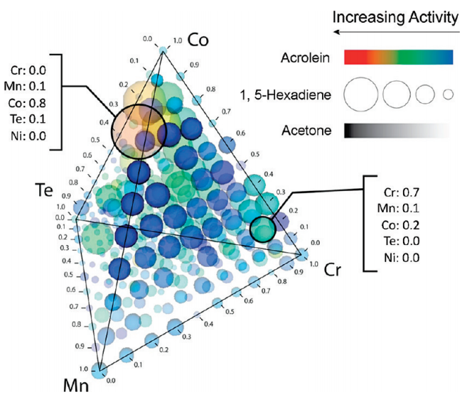
Figure 6.1: 3D glyph plot by Suh et al. (2009).
6.3 Multivariate Data Visualisation Strategies
There are many methods for visualising multivariate data. Strategies for visualising multivariate data can be broken into four main categories, many of which we have already explored in previous chapters.
- Mapping Additional Aesthetics:
ggplot2allows multiple variables to be mapped to different aesthetics. This is a great way to build multivariate representations using standard methods. - Faceting: Faceting breaks a data visualisation into small multiples. This allows the relationship between variables to be considered within the context of another qualitative variable. This strategy is a great way to explore interactions. A simple interaction occurs when a relationship between two variables changes as a result of a third variable.
- Purpose Built: There are many purpose built data visualisations that have been designed specifically for multivariate data. This following chapter will explore a few well-known examples.
- Animation: Animation allows a data visualisation to transition and change usually based on a time variable. Animating a static visualisation provides an additional scale and dimension to the design. Animation will be covered later in Chapters 8 and 9.
The following sections will demonstrate examples of the first three strategies.
6.4 Mapping Additional Aesthetics
The most effective way to visualise multivariate data is to take advantage of ggplot2’s aesthetic mapping by assigning multiple variables to different scales. Deciding which factors are to be the focus should be based on theory, statistical models or hypotheses that the designer wants to visually test (Kirk 2012). Remember to always assign the most accurate scales to the most important variables first. Let’s assume that the relationship between previous education and final grade is the primary focus.
6.4.1 Bivariate
We start with a simple bivariate scatter plot looking at the relationship between gpdPercap and lifeExp using the gapminder dataset. Run the following code to make the Gapminder data available from the gapminder package:
The dataset has the following variables:
- country: Factor with 143 levels
- continent: Factor with 5 levels
- year: ranges from 1952 to 2007 in increments of 5 years
- lifeExp: life expectancy at birth, in years
- pop: population size
- gdpPercap: GDP per capita/per person
Here is a preview of the dataset.
We will filter the data for 2007.
library(dplyr)
gapminder2007 <- gapminder %>% filter(year == 2007)
p1 <- ggplot(gapminder2007, aes(x = gdpPercap, y = lifeExp))
p1 + geom_point() +
  labs(x = "GDP Per Capita", y = "Life Expectancy",
       title = "Country GDP per capita predicts life expectancy (2007)")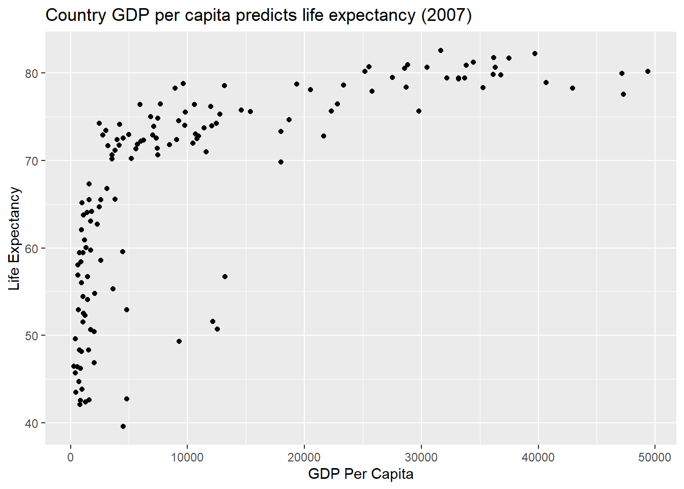
A clear positive, non-linear relationship exists. We can use this basic scatter plot to map additional variables. Let’s start by adding a size = pop aesthetic to produce our first multivariate data visualisation.
6.4.2 Multivariate Visualisation I
p1 + geom_point(aes(size = pop)) +
  labs(x = "GDP Per Capita",
       y = "Life Expectancy",
       title = "Country GDP per capita predicts life expectancy (2007)") +
  scale_size(name = "Pop Size")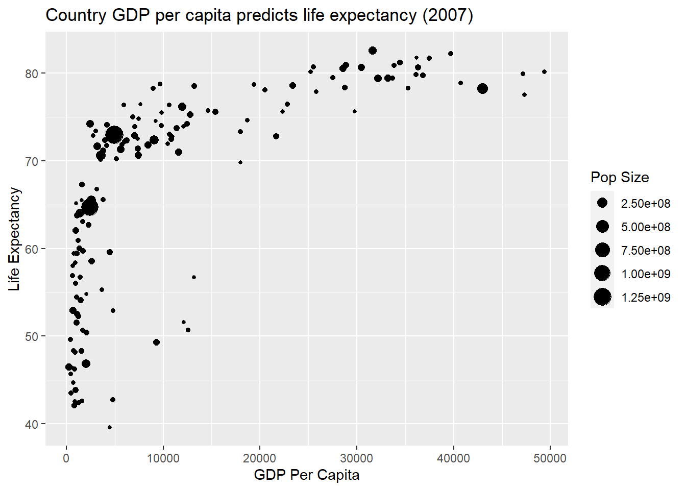
Now the population size of a country is portrayed by the size of the point. Size lacks accuracy, but it does a good job in this example of highlighting the large degree of variability in country size. We will now add a fourth variable. We will map continent to a colour aesthetic.
p1 + geom_point(aes(size = pop, colour = continent)) +
  labs(x = "GDP Per Capita",
       y = "Life Expectancy",
       title = "Country GDP per capita predicts life expectancy (2007)") +
  scale_size(name = "Pop Size") + scale_color_discrete(name = "Continent")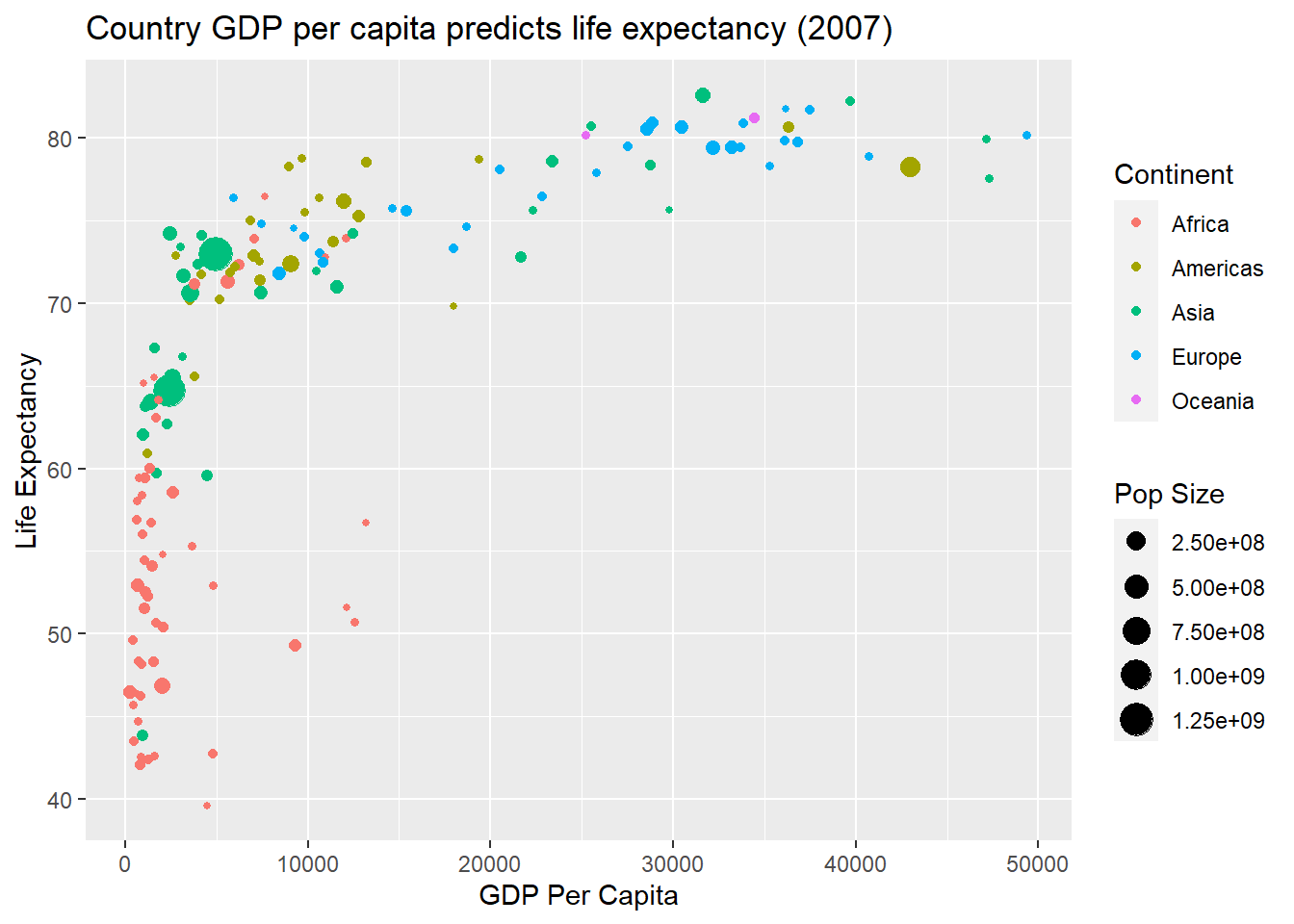
The colour aesthetic does a great job to show major differences in GDP, life expectancy and population size across continents. Colour is a good choice for qualitative variables without a lot of levels.
You might be thinking, “can we add a fifth variable using another aesthetic?” Yes, we can. However, it is not advised. Wickham (2010) suggested that three variable in the same plot is a good rule of thumb.
6.4.3 Learning Analytics Data
We will now turn our attention to the StudentInfo data. The studentInfo dataset (UCI Machine Learning Repository - Open University Learning Analytics Data Set), contains data pertaining to over 30,000 students and their interactions within select courses. In the following chapter, we will use these data to demonstrate strategies for visualising multivariate data.
Specifically, the studentInfo dataset contains the following variables:
- code_module [nominal]: an identification code for a module on which the student is registered
- code_presentation [nominal]: the identification code of the presentation during which the student is registered on the module
- id_student [integer]: a unique identification number for the student
- gender [nominal]: the student’s gender
- region [nominal]: identifies the geographic region where the student lived while taking the module-presentation
- highest_education [nominal]: the student’s highest education level on entry to the module presentation
- imd_band [nominal]: specifies the Index of Multiple Depravation band of the place where the student lived during the module-presentation
- age_band [nominal]: band of the student’s age
- num_of_prev_attempts [integer]: the number of times the student has attempted this module
- studied_credits [integer]: the total number of credits for the modules the student is currently studying
- disability [nominal]: indicates whether the student has declared a disability
- final_result [nominal]: the student’s final result in the module-presentation
studentInfo has been linked and merged with the following two additional variables taken from the studentAssesement dataset (Open University Learning Analytics)
- avg_grade [numeric]: The average grade (out of 100) across all courses
- courses [integer]: The total number of courses completed
Import the data and clean it up. Note how we correct the ordering of the higest_education and final_result variables. Had we not done so, R would order these categories according to alphabetical order.
studentInfo$highest_education <- studentInfo$highest_education %>%
  factor(levels = c("No Formal quals","Lower Than A Level",
                    "A Level or Equivalent", "HE Qualification",
                    "Post Graduate Qualification"),
         ordered = TRUE)

studentInfo$final_result <- studentInfo$final_result %>%
  factor(levels = c("Withdrawn", "Fail", "Pass","Distinction"),
         ordered =TRUE)

studentInfo$gender <- studentInfo$gender %>%
  factor(levels = c("F","M"),
         labels = c("Female","Male"))
Here is a random sample of the full dataset:
6.4.4 Multivariate II
Suppose we are interested in understanding how a student’s previous qualifications, highest_education, is related to avg_grade. We can start with a simple side-by-side box plot.
p2 <- ggplot(data = studentInfo, aes(x = highest_education, y = avg_grade))
p2 + geom_boxplot() +
  labs(y = "Average Grade", x = "Highest Education") +
  coord_flip()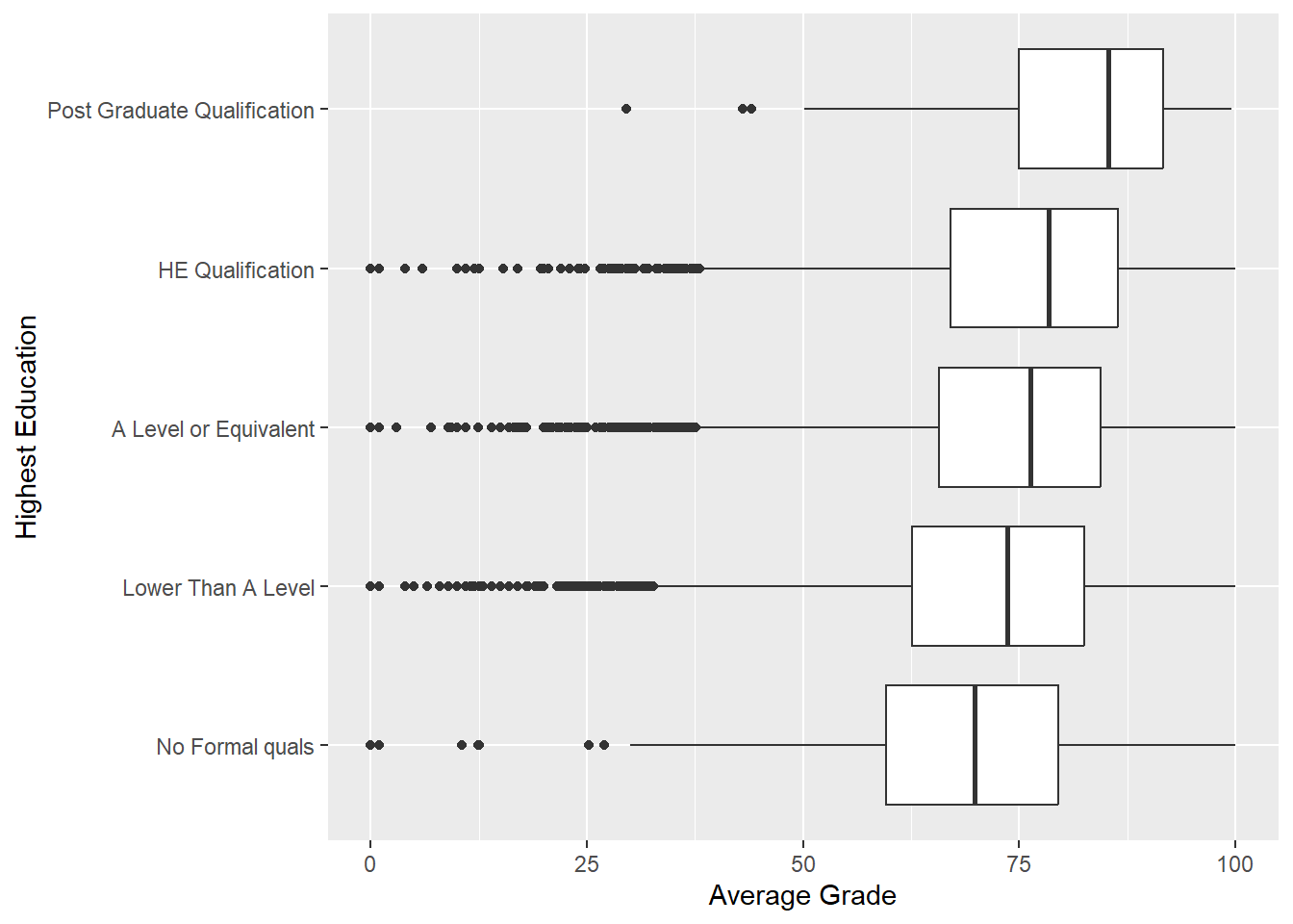
Excellent. There is a nice positive relationship between average grade and highest levels of education. Does this depend on gender?. We can add fill = gender to the aesthetics.
p2 + geom_boxplot(aes(fill = gender)) +
  labs(y = "Average Grade", x = "Highest Education") +
  coord_flip() +
  theme(legend.title=element_blank())
The largely overlapping distributions suggest that there is little difference between males and females on average grades across the different levels of background education. Just with a simple additional aesthetic mapping, ggplot2 can readily produce clear and insightful multivariate data visualisations.
6.4.5 Size
Do students who have higher average grades complete more courses and have higher educational backgrounds? Things are starting to get trickier. This trivariate visualisation includes two quantitative variables and one qualitative variable. The size aesthetic can be used to add an additional quantitative variable. In this visualisation we will map courses to the size aesthetic.
p3 <- ggplot(data = studentInfo,
             aes(x = highest_education, y = avg_grade,
                 size = courses))
p3 + geom_point(position = "jitter",alpha = .25) +
  scale_size(name = "Courses Finished") +
  labs(y = "Average Grade", x = "Highest Education") +
  theme(axis.text.x=element_text(angle=45,hjust=1))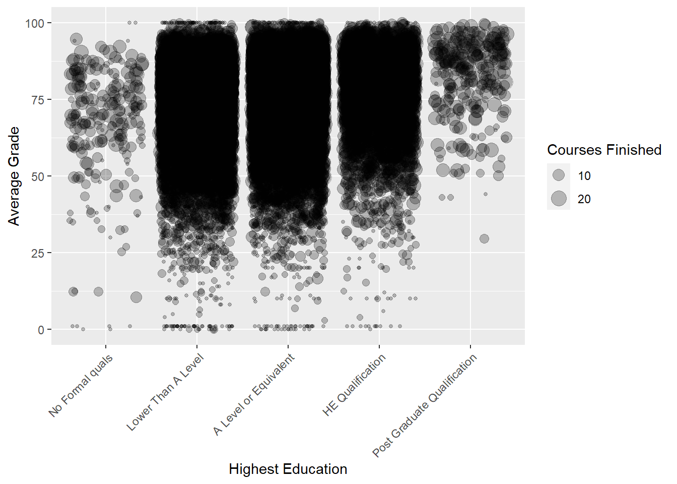
Mixed success. Not all visualisations will work, especially when trying to formulate accurate and intuitive multivariate data visualisations. There are substantial issues with over plotting due to the large sample size. However, we notice two things. First, as a student’s background education level increases, their average grade also increases. Second, focusing on students with no qualifications and post graduate qualifications, there doesn’t appear to be a difference in the number of courses completed, represented as the size aesthetic (note that this does not include students who withdrew). However, I think we would agree that it’s really hard to tell with certainty because the accuracy of the size aesthetic is lacking. We can take a closer look at how the number of courses completed vary by education level using a side-by-side box plot…
p4 <- ggplot(data = studentInfo,
             aes(x = highest_education, y = courses))
p4 + geom_boxplot() +
  labs(y = "Courses Completed", x = "Highest Education") +
  coord_flip()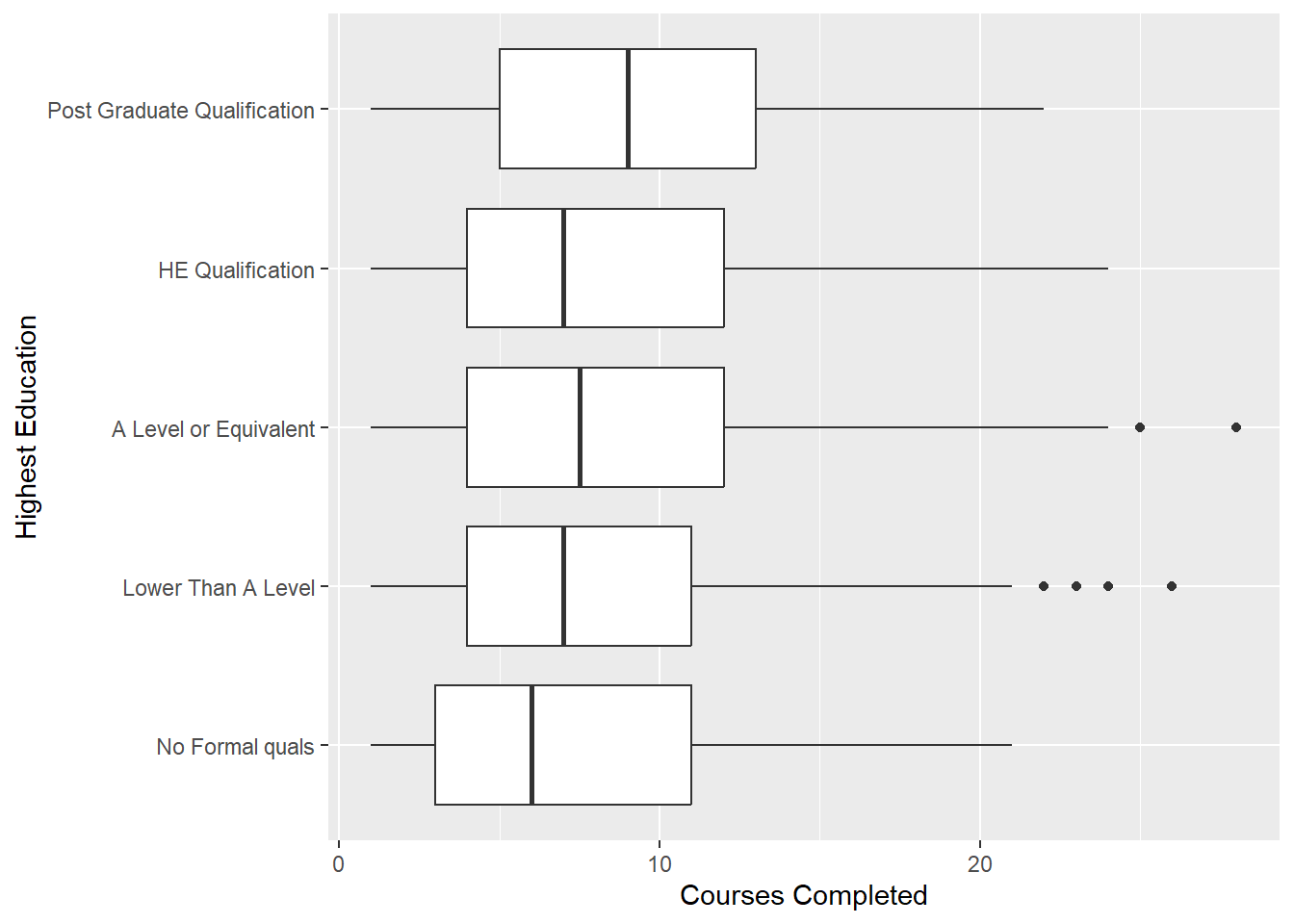
There appears to be a slight increase in the median number of courses completed as level of education increases. We continue our search for a better visualisation…
6.4.6 Colour - Discrete
Perhaps we can visualise the association between avg_grade, highest_education and courses using a different approach. Let’s try mapping highest_education to a colour aesthetic and then place courses on an x-axis and avg_grade on the y-axis. We are careful to select a sequential ColourBrewer scheme to reflect the increasing levels of education. We also add some jitter and transparency to reduce the impact of over-plotting.
p5 <- ggplot(data = studentInfo,
             aes(x = courses, y = avg_grade,colour = highest_education))
p5 + geom_point(position = "jitter") +
  scale_color_brewer(type = "seq", palette = "YlOrRd") +
  labs(y = "Average Grade", x = "Courses Finished")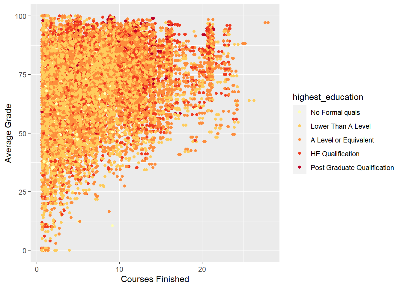
This is a better visualisation. We can see how students with higher average grades tend to finish more courses, and that this trend is somewhat related to highest education. This is reflected in the changing colour. As you move from the bottom left of the plot to the top right, colour changes from yellow to red (higher education. These trends are consistent with the previous plots that have explored the relationships between the number of courses finished, highest education and average grade.
6.4.7 Transforming
The previous visualisation was a vast improvement but it still had issues. One of the main issues was over-plotting. Sometimes a better approach is to transform variables to simplify the data and focus on the main question. We will try transforming course into three equal bands using the cut function.
library(Hmisc)
studentInfo$courses_bands <- studentInfo$courses %>% cut2(g=4, minmax = FALSE)
studentInfo$courses_bands %>% summary()
## [ 1, 5) [ 5, 8) [ 8,12) [12,28] NA's
## 7500 6349 6550 6347 5847The Hmisc::cut2 function creates four approximately equal bands 1 - 4, 5 - 9, 10 - 12 and 13 - 28. There are 5847 missing values. Feeding this into the data visualisation…
studentInfo$courses_bands <- studentInfo$courses_bands %>% factor(
  labels = c("1 - 5",  "6 - 8", "9 - 11", "12 - 28")
)

p6 <- ggplot(data = studentInfo,
             aes(x = highest_education, y = avg_grade,
                 fill = courses_bands))
p6 + geom_boxplot() + scale_fill_brewer(type = "seq",
                                        name = "Courses Completed") +
  coord_flip() + labs(x = "Highest Education", y = "Average Grade")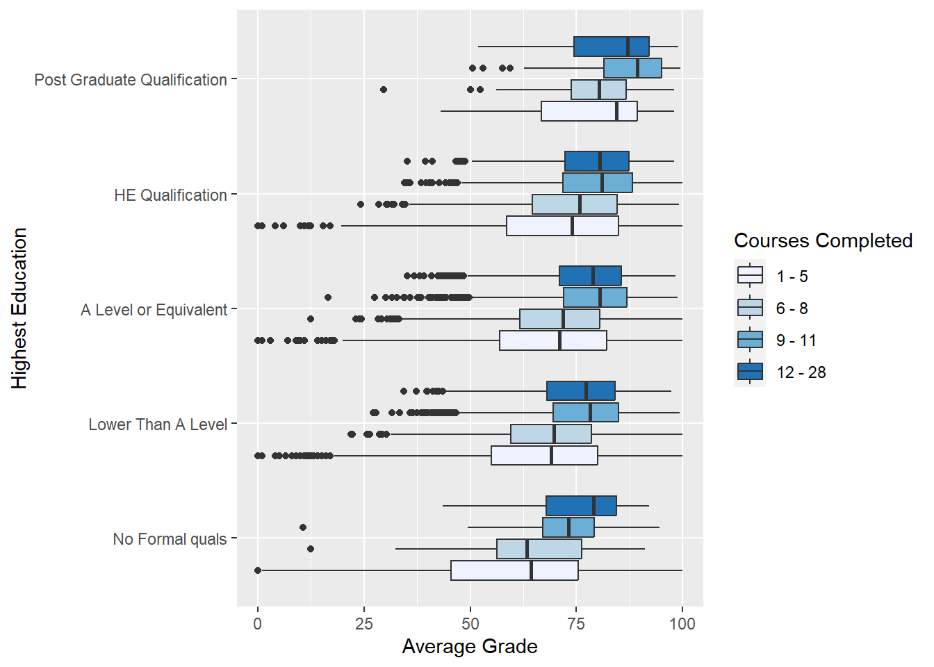
Note the use of the sequential colour scale to represent courses_bands.Students tend to produce higher average grades with when they have higher levels of education and complete more courses. Success breeds success?
6.4.8 Colour- Continuous (Heatmaps)
Continuous colour scales can also be used to rapidly visualise general trends in multivariate data. In the example below, a heat-map generated using the geom_raster() layer in ggplot2 was used to compare average grades across levels of education and region. First, the data were summarised to form a data frame with averages across region and highest level of education.
library(dplyr)
studentInfo_hm <- studentInfo %>% group_by(region, highest_education)
studentInfo_hm <- studentInfo_hm %>% summarise(count = n(),
                                               mean = mean(avg_grade, na.rm = TRUE))
Here is the result:
Now we generate the heat-map.
p7 <- ggplot(data = studentInfo_hm, aes(x = highest_education,
                                     y = region,
                                     fill = mean))
p7 + geom_raster() + labs(y = "Region", x = "Highest Education") +
  scale_fill_continuous(name="Average\nGrade") +
   theme(axis.text.x=element_text(angle=45,hjust=1))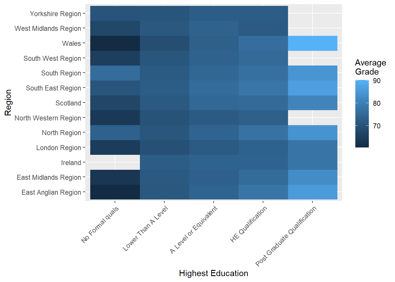
Some ordering would be an improvement. Let’s try ordering regions from best to worst performing. First, calculate the mean grade by region in order to rank.
performance <- studentInfo %>% group_by(region) %>%
  summarise(mean = mean(avg_grade, na.rm = TRUE))
performance %>% arrange(mean)
## # A tibble: 13 × 2
## region mean
## <chr> <dbl>
## 1 London Region 71.1
## 2 North Western Region 71.1
## 3 Yorkshire Region 71.6
## 4 Wales 71.9
## 5 West Midlands Region 72.4
## 6 South West Region 72.6
## 7 East Midlands Region 72.7
## 8 East Anglian Region 73.2
## 9 Ireland 73.4
## 10 South Region 73.8
## 11 North Region 73.8
## 12 Scotland 74.4
## 13 South East Region 74.7We then order the region factor by the mean ranks using the dplyr::arrange function.
studentInfo_hm$region <- studentInfo_hm$region %>%
  factor(levels = arrange(performance,mean)$region)
Re-plotting…
p7 <- ggplot(data = studentInfo_hm, aes(x = highest_education,
                                     y = region,
                                     fill = mean))

p7 + geom_raster() + labs(y = "Region", x = "Highest Education") +
  scale_fill_continuous(name="Average\nGrade") +
   theme(axis.text.x=element_text(angle=45,hjust=1))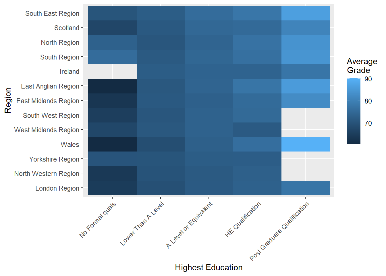
This visualisation can be used to rapidly identify regions that exhibit strong relationships between highest education and average grades. For example, Wales and East Anglian appear to have the strongest relationship between education and average grade. This is represented by the incremental change in colour value across levels of highest education (from dark to light). In contrast, Yorkshire and Ireland show very little variability because colour almost stays the same across highest education levels.
Heat-maps are great for identifying broad trends, however, they lack substantial accuracy because a continuous colour scale is being used to represent a quantitative variable. Subtle changes in colour may make it more difficult to perceive variation in the quantitative variable.
6.5 Faceting
In the previous sections, we added various aesthetic mappings to build multivariate displays. However, in most cases we are restricted in the number of variables that we can accurately map and visualise. When we hit the practical and perceptual limitations of mapping aesthetics, we can overcome the issues of over-plotting by exploiting the power of faceting. Faceting is the process of breaking data visualisations into small multiples. It is also called latticing or trellising.
Let’s explore the use of facets to visualise the relationship between highest education, gender and average grades by region. That’s four variables in total. This visualisation might be helpful to determine how the background of students from different regions might interact with the relationships between the other variables. The beauty of facets in ggplot2 is that they are really easy to do.
6.5.1 Single Facet
Let’s build the combined plot:
p8 <- ggplot(data = studentInfo, aes(x = highest_education,
                                         y = avg_grade,
                                         fill = gender))
p8 + geom_boxplot() + labs(y = "Average Grade", x = "Highest Education") +
  theme(legend.title=element_blank()) + coord_flip()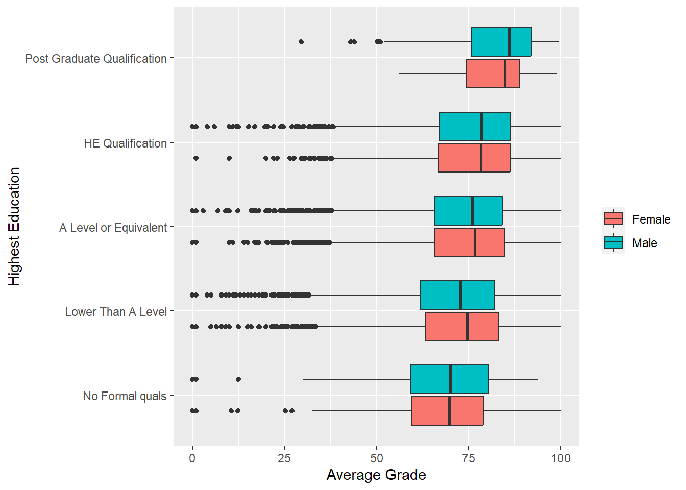
Easy. Now for the fun part…
p8 + geom_boxplot() + labs(y = "Average Grade", x = "Highest Education") +
  theme(legend.title=element_blank()) + coord_flip() +
  facet_wrap(~ region)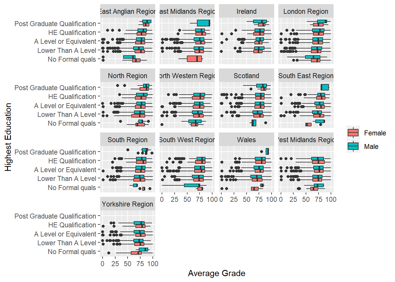
There are a few facet options in ggplot2 including facet_wrap and facet_grid. facet_wrap will automatically generate a two-dimensional grid of plots which is perfect for making the most of space. However, if you want to align visualisations as rows or columns to facilitate accurate comparisons you can use facet_grid. The facet_grid function uses an expression, . ~ ., to determine if a variable appears as rows or columns. The left-hand side of the tilde symbol refers to rows and the right hand side to columns. For example, facet_grid(. ~ var) will align facets as columns and facet_grid(var ~ .) as rows.
p8 + geom_boxplot() + labs(y = "Average Grade", x = "Highest Education") +
  theme(legend.title=element_blank()) + coord_flip() +
  facet_grid(region ~ .)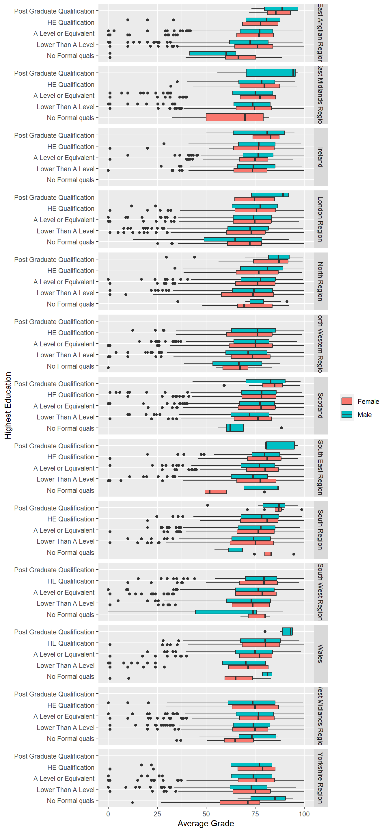
6.5.2 Double Facet
If you dare and you have a really big screen, you can also do double facets. However, as you break the data up into smaller and smaller facets, you will start to have issues fitting everything in even on the biggest of screens and also with empty facets. Use with caution. As a rule of thumb, you should never use more than two variables in a facet.
p8 + geom_boxplot() + labs(y = "Average Grade", x = "Highest Education") +
  theme(legend.title=element_blank()) + coord_flip() +
  facet_grid(region ~ age_band)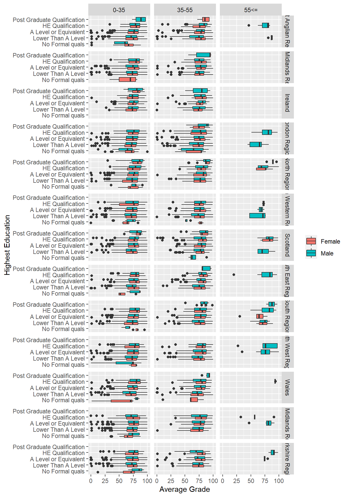
6.5.3 Emphasis
Deciding to use rows or columns is an important decision as it will impact the comparisons emphasised. The infographic in Figure 6.2) explains the rules. Facets aligned as columns makes comparisons on the y-axis quick and accurate. Facets aligned as rows emphasise comparisons on the x-axis. Making comparison across un-aligned panels are harder and less accurate. Ensure the most important comparison you want the audience to make are easy and accurate by choosing rows and columns appropriately.
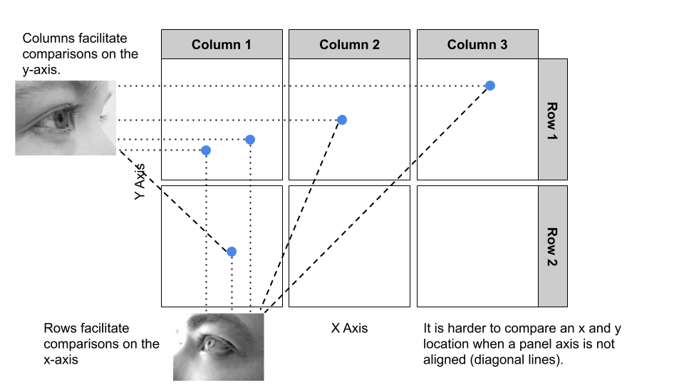
Figure 6.2: Aligning facets as rows or columns impacts the ease and accuracy of comparisons across panels.
6.6 Purpose Built
There are many purpose built data visualisations that have been designed exclusively for multivariate data. We will take a look at a few common examples, however, there are much more examples in the field of data visualisation to explore.
6.6.1 Sankey Diagrams
Sankey diagrams are excellent visualisations for displaying data flow. They date back to 1812 when Charles Minard published a famous visualisation of Napoleon’s Russian Campaign (Figure 6.3).
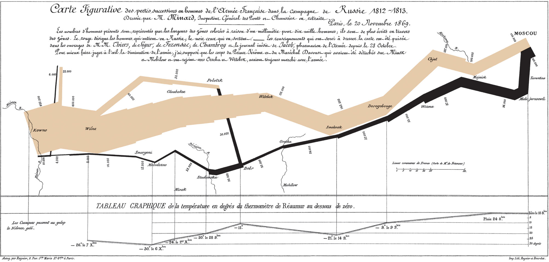
Figure 6.3: Charles Minard’s famous visualisation of Napoleon’s Russian Campaign (Minard 1869).
However, their name is attributed to Captain Matthew Henry Phineas Riall Sankey who in 1898 published a Sankey diagram showing the flow of energy through a steam engine (see Figure 6.4).
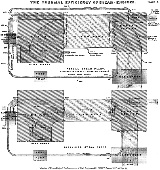
Figure 6.4: The thermal efficiency Of steam engines by Sankey (1898).
As we will see, these very old visualisations are still useful today. I must thank my student Krishna Dermawan for showing me how to produce these visualisations in R. Krishna did a lot of work figuring out how to clean and structure the data for these types of diagrams. We will produce a Sankey diagram using the googleVis package. Ensure you install and load the package:
library(googleVis)Krishna used Sankey diagrams for a very useful purpose in a consultancy he did for the Design & Social Context College at RMIT University. The college wanted a way to visualise student preference data (i.e. 1st, 2nd, 3rd, and 4th) with a focus on post-graduate teaching programs. Student university preferences are managed by Victorian Tertiary Admissions Centre (VTAC) and the data are available to universities. Krishna’s first job was to clean and restructure the data. The fruits of his hard work are captured in the StudentPreference. The variables are as follows:
- ID [Integer]:
- Pref_1 [Factor]: 1st preference: ACU, Deakin, FedUni, LaTrobe, Monash, RMIT, UniofMelb, Unknown, VicUni
- Pref_2 [Factor]: 2nd preference: ACU, Deakin, FedUni, LaTrobe, Monash, RMIT, UniofMelb, Unknown, VicUni
- Pref_3 [Factor]: 3rd preference: ACU, Deakin, FedUni, LaTrobe, Monash, RMIT, UniofMelb, Unknown, VicUni
- Pref_4 [Factor]: 4th preference: ACU, Deakin, FedUni, LaTrobe, Monash, RMIT, UniofMelb, Unknown, VicUni
StudentPreference<-read.csv("data/StudentPreference.csv")Here is the preview of the dataset:
The StudentPreference dataset needs to be converted to flow data. These are represented as cross tabulations showing the relationships Pref_1 and Pref_2, Pref_2 and Pref_3, and Pref_3 and Pref_4. Each variable represents a node and the counts are the flow of data to the next variable.
StudentPreference_sk_1 <- table(StudentPreference$Pref_1,
                                   StudentPreference$Pref_2)
StudentPreference_sk_2 <- table(StudentPreference$Pref_2,
                                   StudentPreference$Pref_3)
StudentPreference_sk_3 <- table(StudentPreference$Pref_3,
                                   StudentPreference$Pref_4)
We also convert these tables into data.frame objects.
StudentPreference_sk_1 <- data.frame(StudentPreference_sk_1)
StudentPreference_sk_2 <- data.frame(StudentPreference_sk_2)
StudentPreference_sk_3 <- data.frame(StudentPreference_sk_3)
We need to be careful about how we label each university. Because each university will be repeated in each connecting node, Pref_1, gvisSankey() will get confused. We need to append each label with a number that anchors it to the order of preferences. For example 1. UniofMelb refers to the first preference and 2. UniofMelb refers to the 2nd preference.
StudentPreference_sk_1$Var1 <- paste("1.",StudentPreference_sk_1$Var1)
StudentPreference_sk_1$Var2 <- paste("2.",StudentPreference_sk_1$Var2)

StudentPreference_sk_2$Var1 <- paste("2.",StudentPreference_sk_2$Var1)
StudentPreference_sk_2$Var2 <- paste("3.",StudentPreference_sk_2$Var2)

StudentPreference_sk_3$Var1 <- paste("3.",StudentPreference_sk_3$Var1)
StudentPreference_sk_3$Var2 <- paste("4.",StudentPreference_sk_3$Var2)gvisSankey, the function we will call to generate the diagram, requires the data to be in a dataset with three variables, from, to and weight. The following code will join the three converted data.frame objects above into a single object.
StudentPreference_sk<-rbind(StudentPreference_sk_1,StudentPreference_sk_2,StudentPreference_sk_3)Here is the preview of the restructured data.
We will use Var1 to represent our from variable, Var2 for our to variable and Freq as our weight. We can then construct the Sankey diagram.
sk1 <- gvisSankey(StudentPreference_sk, from='Var1', to='Var2', weight='Freq',
                options=list(height=600, width=800))

plot(sk1)
We can use this diagram to visually explore trends in how students are allocating their preferences.
Krishna warns that as of March 2016, Sankey diagrams created using googleVis have a number of limitations:
- The vertical ordering of each category (“nodes”) within a ranking cannot be customised
- The individual cannot choose a colour scheme for each node or the flow (“link”).
- Most importantly, the
gvisSankey()function does not allow the same nodes to be repeated within the flow.
Let’s take a look at another interesting example.
The msnbc dataset, taken from the UCI Machine Learning Repository, contains the sequence of page view categories for over 1 million unique visitors to the MSNBC.com website logged on the 28th of September, 1999. The categories, or different landing pages, included: “frontpage”, “news”, “tech”, “local”, “opinion”, “on-air”, “misc”, “weather”, “health”, “living”, “business”, “sports”, “summary”, “bbs” (bulletin board service), “travel”, “msn-news”, and “msn-sports”. A Sankey diagram is a great way to visualise how visitors interact with different sections of the site within a 24-hour period. As we will discover, there are some really interesting visitor patterns.
msnbc <- read.csv("msnbc.csv")Here is a random preview of the dataset.
There is quite a bit of data-preprocessing required because there are 17 different page categories. A Sankey diagram cannot present the flow between this many categories. The first step will be to group the less common page categories into an “other” category. First, we will convert msnbc to a long format using the tidyr::gather() function. This will make it easier to work with the page categories.
library(tidyr)
msnbc_l <- msnbc %>%
  gather(key = "Visit", value = "Page", 1:10, na.rm = FALSE)
For some reason, the gather() function converts factors to strings. Let’s change them back.
msnbc_l <- msnbc_l %>% lapply(factor) %>% data.frame()Now let’s produce a frequency distribution of page categories.
msnbc_tbl <- table(msnbc_l$Page) %>% data.frame()
msnbc_tbl %>% arrange(-Freq)
## Var1 Freq
## 1 frontpage 940469
## 2 news 452387
## 3 weather 439398
## 4 on-air 414928
## 5 bbs 395880
## 6 local 386217
## 7 misc 305615
## 8 sports 264899
## 9 summary 216125
## 10 tech 207479
## 11 health 196614
## 12 opinion 151409
## 13 living 131760
## 14 business 96817
## 15 travel 56576
## 16 msn-news 25249
## 17 msn-sports 16972Visually…
library(forcats)
ggplot(msnbc_tbl, aes(x = Freq, y = fct_reorder(Var1,Freq))) +
  geom_point()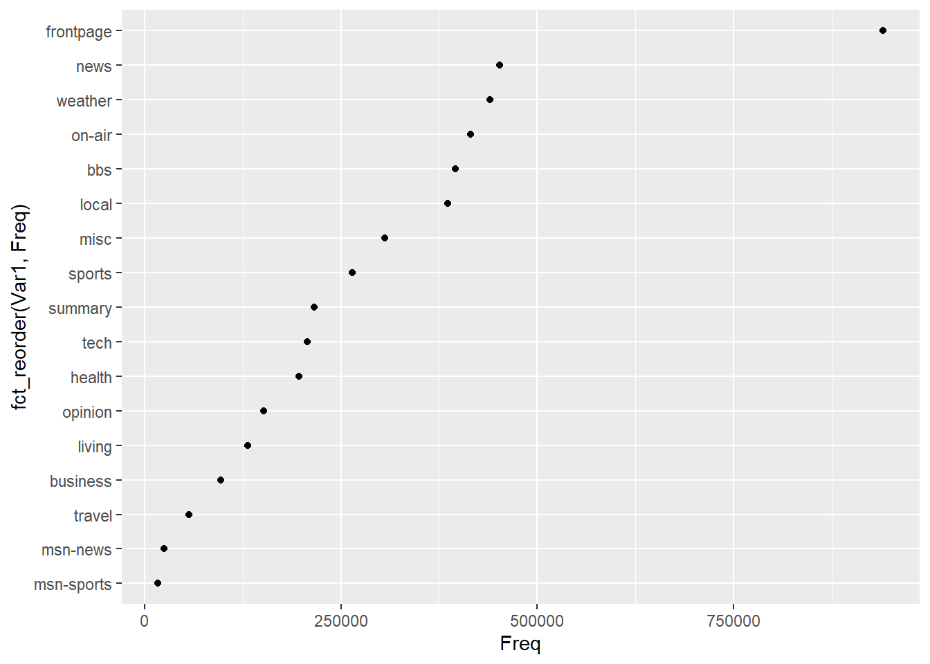
We used the forcats::fct_reorder function to rank the page categories in the dot plot. We can see that the front page, news, weather, on-air and bbs are the top 5 categories. We will stick to the top five as this will give us good insight into how the majority of users move around the site.
We can use the dplyr::mutate, dplyr::across and forcats::fct_collapse functions to quickly re-code the original page categories to the top five and a “other” category. First, let’s ensure the factors are configured in msnbc.
str(msnbc)## 'data.frame': 1153752 obs. of 10 variables:
## $ First : chr "frontpage" "news" "tech" "opinion" ...
## $ Second : chr "frontpage" NA "news" NA ...
## $ Third : chr NA NA "news" NA ...
## $ Fourth : chr NA NA "local" NA ...
## $ Fifth : chr NA NA "news" NA ...
## $ Sixth : chr NA NA "news" NA ...
## $ Seventh: chr NA NA "news" NA ...
## $ Eighth : chr NA NA "tech" NA ...
## $ Ninth : chr NA NA "tech" NA ...
## $ Tenth : chr NA NA NA NA ...msnbc <- data.frame(lapply(msnbc,factor))
str(msnbc)## 'data.frame': 1153752 obs. of 10 variables:
## $ First : Factor w/ 17 levels "bbs","business",..: 3 10 15 12 3 11 3 11 11 11 ...
## $ Second : Factor w/ 17 levels "bbs","business",..: 3 NA 10 NA NA NA 3 NA 7 4 ...
## $ Third : Factor w/ 17 levels "bbs","business",..: NA NA 10 NA NA NA NA NA 7 6 ...
## $ Fourth : Factor w/ 17 levels "bbs","business",..: NA NA 6 NA NA NA NA NA 7 6 ...
## $ Fifth : Factor w/ 17 levels "bbs","business",..: NA NA 10 NA NA NA NA NA 11 6 ...
## $ Sixth : Factor w/ 17 levels "bbs","business",..: NA NA 10 NA NA NA NA NA 11 5 ...
## $ Seventh: Factor w/ 17 levels "bbs","business",..: NA NA 10 NA NA NA NA NA 17 15 ...
## $ Eighth : Factor w/ 17 levels "bbs","business",..: NA NA 15 NA NA NA NA NA 17 5 ...
## $ Ninth : Factor w/ 17 levels "bbs","business",..: NA NA 15 NA NA NA NA NA 17 12 ...
## $ Tenth : Factor w/ 17 levels "bbs","business",..: NA NA NA NA NA NA NA NA 17 5 ...The following code uses dplyr::across to apply the forcats::fct_collapse function in order to change, or “mutate” the original values in each column of msnbc. The top five categories are retained, and all other categories are “lumped” into other_levels. This mutated data frame is saved as msnbc_lumped.
library(dplyr)
library(forcats)
msnbc_lumped <-
  msnbc %>%  mutate(across(First:Tenth,
    ~ forcats::fct_collapse(.x,
      bbs = "bbs",
      frontpage = "frontpage",
      news = "news",
      onair = "on-air",
      weather = "weather",
      other_level = "other"
    )
  ))

summary(msnbc_lumped)
## First Second Third Fourth
## bbs : 68605 bbs : 64742 bbs : 54738 bbs : 46811
## frontpage:306151 frontpage:143752 frontpage:108452 frontpage: 87163
## news : 93067 news : 77794 news : 61795 news : 50894
## onair :173170 onair : 56710 onair : 39301 onair : 30110
## weather : 85828 weather : 70381 weather : 58873 weather : 51486
## other :426931 other :356321 other :276985 other :222754
## NA's :384052 NA's :553608 NA's :664534
## Fifth Sixth Seventh Eighth
## bbs : 38942 bbs : 32950 bbs : 27866 bbs : 23687
## frontpage: 71634 frontpage: 58876 frontpage: 50772 frontpage: 43230
## news : 41190 news : 34515 news : 28896 news : 24604
## onair : 29639 onair : 22708 onair : 20488 onair : 16882
## weather : 44942 weather : 36804 weather : 29552 weather : 24490
## other :181149 other :155569 other :131184 other :114625
## NA's :746256 NA's :812330 NA's :864994 NA's :906234
## Ninth Tenth
## bbs : 20176 bbs : 17363
## frontpage: 37639 frontpage: 32800
## news : 21220 news : 18412
## onair : 14033 onair : 11887
## weather : 20234 weather : 16808
## other :100732 other : 89482
## NA's :939718 NA's :967000Excellent. We can now prepare the data for visualisation. As we have 10 nodes to connect, we can use a loop to build the required data.frame. In this loop, we need to create unique nodes when a factor level repeats. For example, “frontpage” –> “frontpage” will confuse the function. Instead, we can use a unique name to maintain the “flow” in the data. For example, we can use “p. 1: frontpage” –> “p. 2: frontpage”. Pay close attention to the paste function below.
msnbc_sk <- data.frame()

for (i in 1:9){
  msnbc_sub <- msnbc_lumped
  levels(msnbc_sub[,i]) <- paste("p.",i,": ",levels(msnbc_sub[,i]), sep = "")
  levels(msnbc_sub[,i+1]) <- paste("p.",i+1,": ",levels(msnbc_sub[,i+1]), sep = "")
  df <- table(msnbc_sub[,i],msnbc_sub[,i+1])
  msnbc_sk<-rbind(msnbc_sk,df)
}
And the result:
Next, the easy part…
sk2<-gvisSankey(msnbc_sk, from='Var1', to='Var2', weight='Freq',
                options=list(height=400, width=800,  title="Diagram Title"))

plot(sk2)
The diagram shows a powerful trend. It appears that most visitors stay within the same page categories, with very few exploring other areas of the site. This suggests distinct clusters of users, but also indicates there is a great opportunity to propose website changes that encourage visitors to explore other sections.
6.6.2 Parallel Coordinates
In a parallel coordinate system, a visualisation popularised by Alfred Inselberg (1985), each variable is mapped to an evenly spaced series of vertical axes. Each vertical axis represents a single variable and connecting lines are used to visualise the relationship between adjacent variables. Each variable’s scale is transformed so that all vertical lines share the same height. This method allows multivariate relationships to be represented using a 2D plane. The following visualisation provides an example.
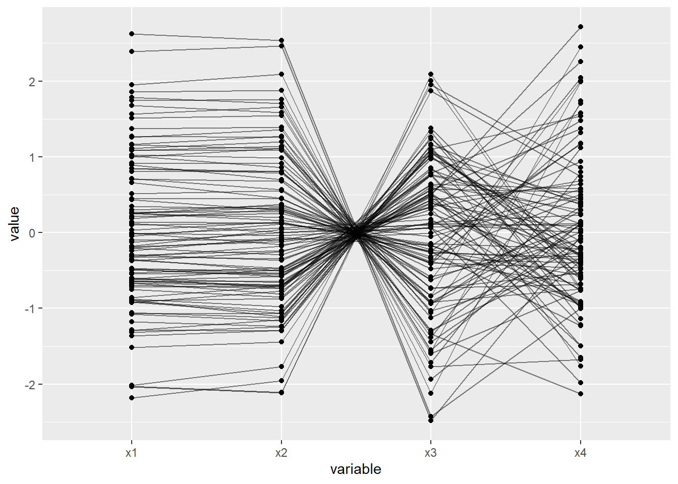
Here is a description of each relationship depicted:
- x1–>x2: Strong positive linear relationship
- x2–>x3: Strong negative linear relationship
- x3–>x4: No relationship
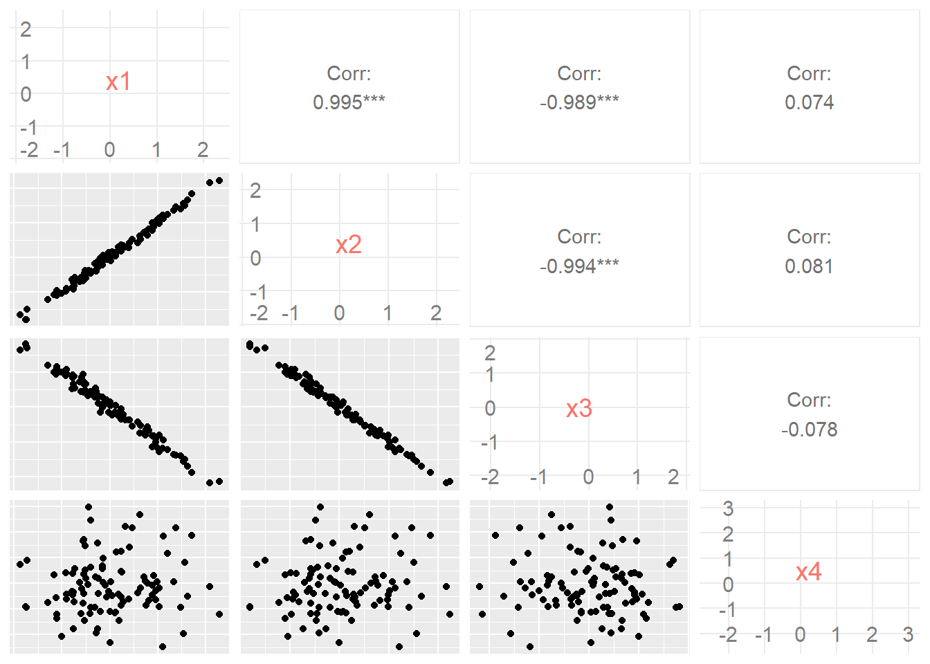
Note that we have four variables, but only three relationships are visualised. This is a limitation of parallel coordinate systems. With 4 variables, we have \({4 \choose 2} = 6\) possible bivariate relationships to explore. This is better served using a matrix scatter plot.
We can create a parallel coordinates plot using the GGally package and the Body data. The Body dataset contains the percentage of body fat, age, weight, height, and 10 body circumference measurements (e.g., abdomen) for a sample of 252 men. Variables include the following:
- Case [Integer]: Case Number
- BFP_Brozek [Numeric]: Percent body fat using Brozek’s equation, 457/Density - 414.2
- BFP_Siri [Numeric]: Percent body fat using Siri’s equation, 495/Density - 450
- Density [Numeric]: Density (gm/cm3)
- Age [Integer]: Age (yrs)
- Weight [Numeric]: Weight (lbs)
- Height [Numeric]: Height (inches)
- Adiposity_index [Numeric]: Adiposity index = Weight/Height2 (kg/m2)
- Fat_free [Numeric]: Fat Free Weight = (1 - fraction of body fat) * Weight, using Brozek’s formula (lbs)
- Neck [Numeric]: Neck circumference (cm)
- Chest [Numeric]: Chest circumference (cm)
- Abdomen [Numeric]: Abdomen circumference (cm) “at the umbilicus and level with the iliac crest”
- Hip [Numeric]: Hip circumference (cm)
- Thigh [Numeric]: Thigh circumference (cm)
- Knee [Numeric]: Knee circumference (cm)
- Ankle [Numeric]: Ankle circumference (cm)
- Biceps [Numeric]: Extended biceps circumference (cm)
- Forearm [Numeric]: Forearm circumference (cm)
- Wrist [Numeric]: Wrist circumference (cm) “distal to the styloid processes”
Here is a preview of the dataset.
Now let’s explore the relationship between BFP_Siri, Abdomen, Weight and Height. We will use this visualisation to show why body fat is best indicated by an abdomen measurement as opposed to weight, which is better determined by a person’s height.
library(GGally)
ggparcoord(data = Body, columns = c(3, 12, 6, 7))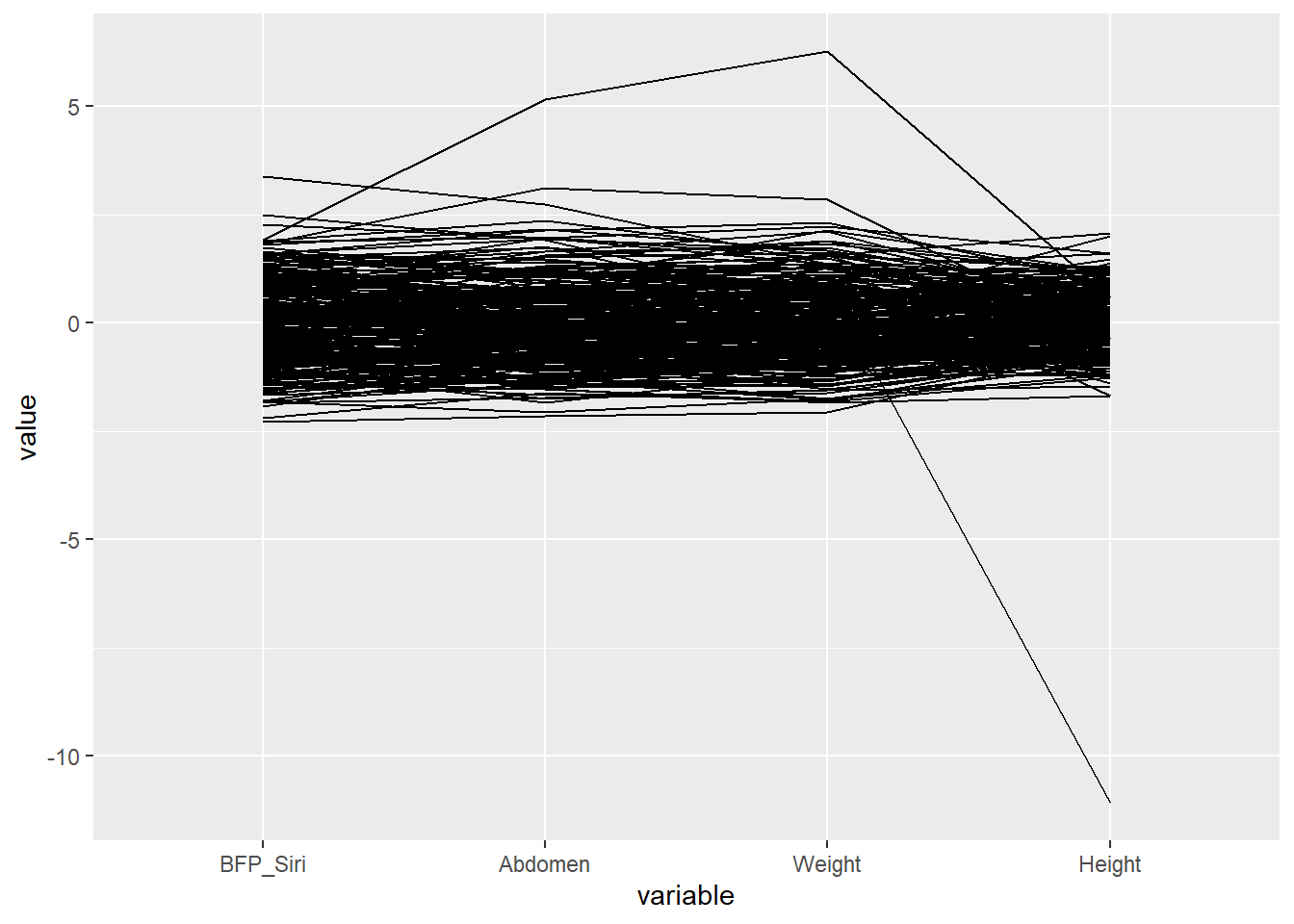
That outliers needs addressing:
ggparcoord(data = filter(Body, Height > 40 & Abdomen < 140),
           columns = c(3, 12, 6, 7))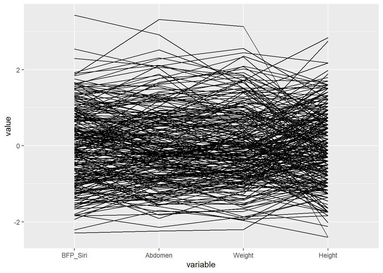
To help you interpret the visualisation, use the following matrix.
ggpairs(filter(Body, Height > 40 & Abdomen < 140),
        columns = c(3, 12, 6, 7), axisLabels = "internal")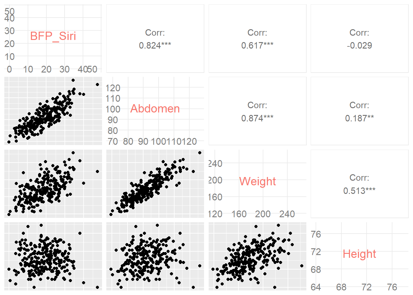
We can also add colour to represent groups. For example, we can colour lines based on age categories.
Body <- mutate(Body, Age_cat = ifelse(Age < 40,"22 - 39","40+"))

ggparcoord(data = filter(Body, Height > 40 & Abdomen < 140),
           columns = c(3, 12, 6, 7), groupColumn = 20)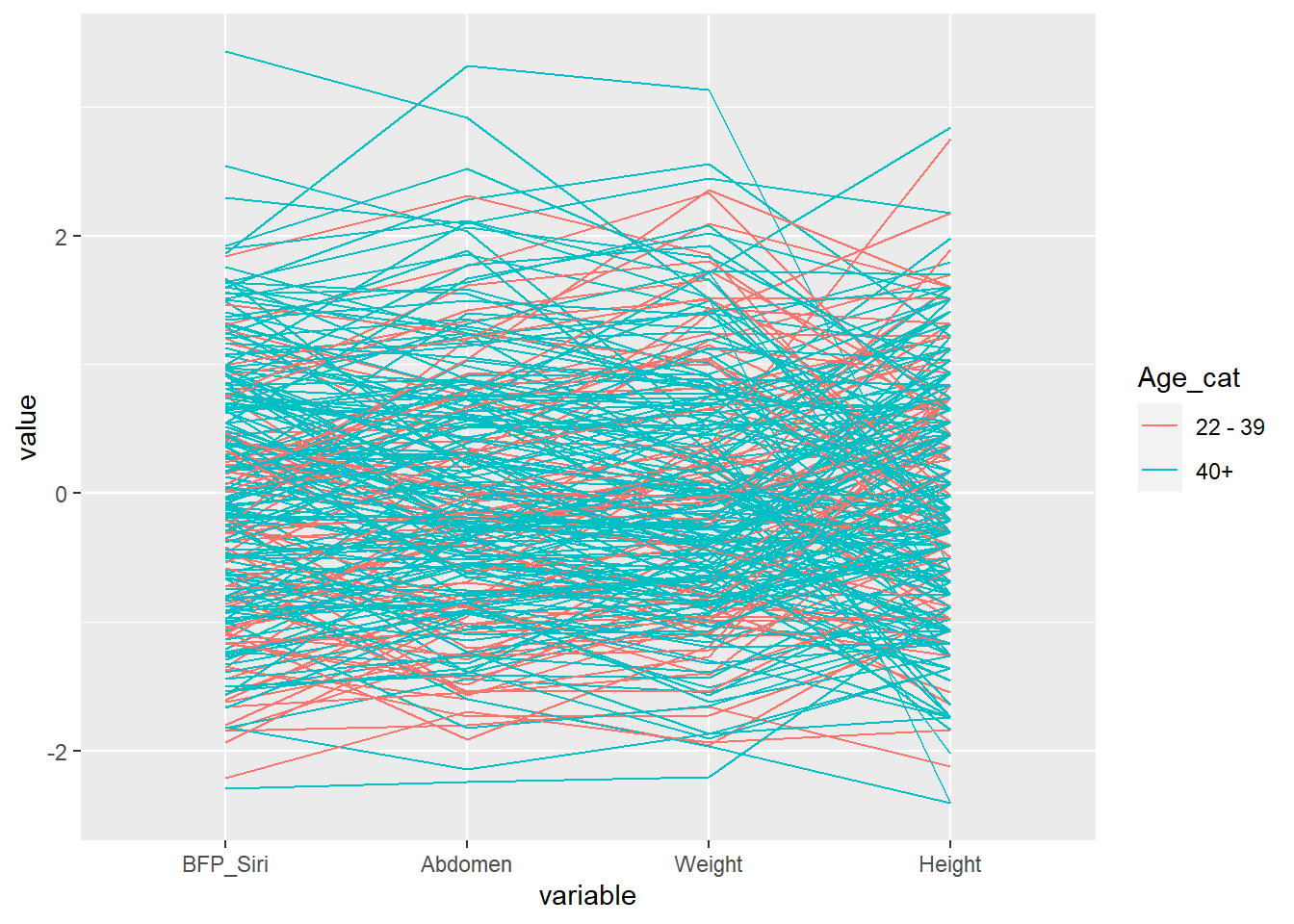
Parallel coordinate systems are a variation of a scatter plot matrix, however, they are limited by only being able to show relationships between adjacent variables. Therefore, the designer needs to think carefully about how to best order the variables to tell the story behind the data. They also take a bit of training to interpret. I feel scatter plots are more intuitive.
ggpairs(filter(Body, Height > 40 & Abdomen < 140), ggplot2::aes(colour = Age_cat),
        columns = c(3, 12, 6, 7),axisLabels = "internal")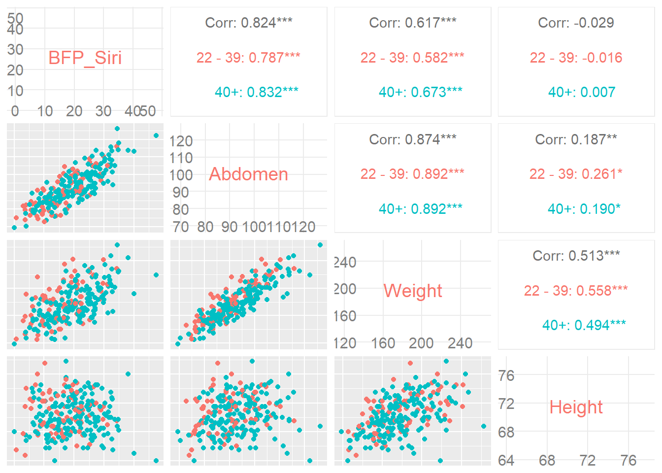
6.6.3 3D Scatter Plots
ggplot2 does not create 3D scatter plots and many of the R packages that do so are based on outdated technology used to generate interactive features. We will make use of the very powerful plotly package (Plotly), which will be fully explored in a later chapter. Plotly is producing some seriously awesome data visualisation tools that essentially aim to provide a common method to translate data visualisations produced using leading data visualisation tools into D3.js objects. What does this mean? Really awesome interactive plots that can be easily integrated in webpages. No more static plots! Let’s give it a crack. Ensure you install and load the plotly package first.
We will visualise the interrelationships between Weight, Height and BF_Siri using the Body dataset.
library(plotly)
library(dplyr)

Body_filt <- filter(Body, Height > 50) #Remove outlier
plot_ly(data = Body_filt, x = ~Height, y = ~Weight, z = ~BFP_Siri) %>% add_markers()
After the plot appears in the RStudio Viewer, click the “Show in new Window” button. This will load the 3D scatter plot in a web browser, which is exactly how you want to view this baby, in all its interactive glory. You can click and rotate the axes. You can also use the Plotly tool bar to explore a static plot image, zoom, rotate, pan and alter various other options. Don’t worry. You will get to spend a complete chapter exploring Plotly further. Eventually we will push these plots onto the Plotly server for the world to see.
As cool as these visualisations are, they do assume you can interact with the plot to make sense of the interrelationships. Without interaction, you are forced to view the plot from one angle. As you are trying to visualise three dimensions using a two-dimensional space, these plots can become very difficult to interpret. You are better to stick with producing a matrix scatterplot as detailed in Chapter 5.
6.6.4 Multivariate Mosaic Plots
Mosaic plots, covered previously in the Chapter 5 Grammar and Vocabulary chapter, can also be extended to visualise three qualitative variables. Let’s jump back to the studentInfo dataset and produce one for the visualisation looking at highest_education, final_result and gender. Note we have to shorten the factor labels to ensure all the labels fit into the plot.
library(vcd)
studentInfo <- read.csv("data/studentInfo.csv")
studentInfo$highest_education <- factor(studentInfo$highest_education,
                                        levels = c("No Formal quals","Lower Than A Level",
                                                   "A Level or Equivalent", "HE Qualification",
                                                   "Post Graduate Qualification"),
                                        labels = c("None","< A Level",
                                                   "A Level", "HE",
                                                   "PG"),
                                        ordered = TRUE)

studentInfo$final_result <- factor(studentInfo$final_result,
                                   levels = c("Withdrawn", "Fail", "Pass","Distinction"),
                                   labels = c("WD", "F", "P","D"),
                                   ordered =TRUE)

studentInfo$gender <- factor(studentInfo$gender, levels = c("F","M"),
                             labels = c("F","M"))

mosaic(~ highest_education + final_result | gender,
       data = studentInfo,
       labeling_args = list(set_varnames =
                              list(final_result =
                                     "Final Results",
                                   highest_education = "Highest Education",
                                   gender = "Gender")),
       shade=TRUE, legend=TRUE)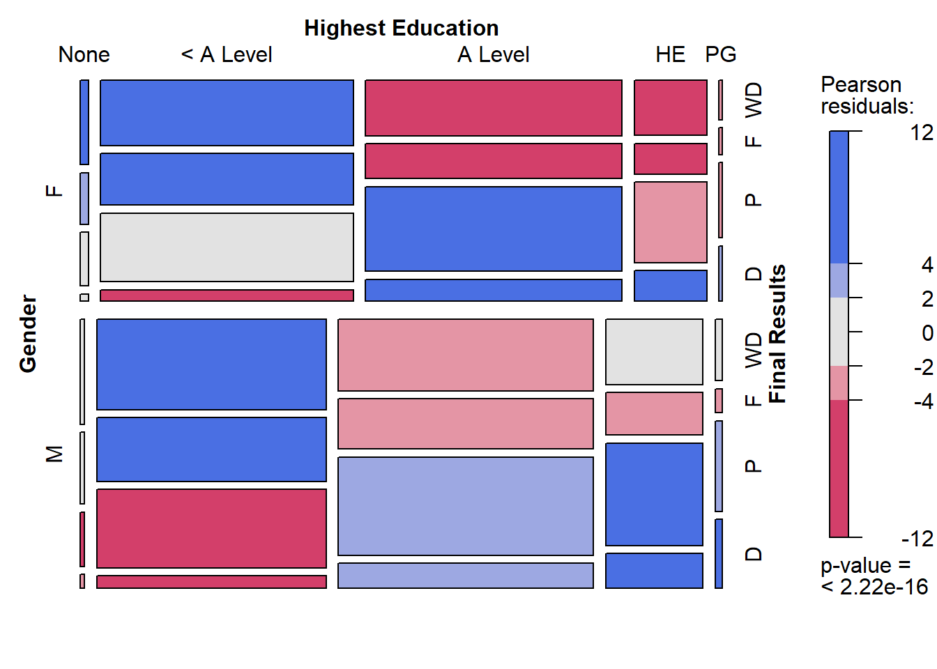
This Mosaic plot compares males and females on the association between highest edcuation and final_result. Try to observe the following visual points:
- Students enrolling with no education background were more likely to be female.
- Students enrolling with post graduate qualifications were more likely to be male.
- Males and females with < A level education were overrepresented in the ‘fail’ and ‘withdrawn’ final result categories.
- Males, but not females, with < A level education were under-represented in the passing of the course.
- Males who have completed higher education and post graduate qualifications were more likely to pass or gain a distinction than females with the same levels of education.
This powerful visualisation tells many more stories, but as you will find they take quite a bit of effort to perceive. Therefore, you won’t see multivariate mosaic plots used very often and you should avoid using them for general audiences.
6.7 Concluding Thoughts
This chapter discussed strategies for visualising multivariate data. Due to the limitations of human perception, multivariate data visualisations must be carefully designed. The strategies discussed included mapping additional aesthetics, facets, and purpose built. The fourth strategy, animation will be introduced in later chapters. You now have the basic strategies under your belt. These will help you to design accessible multidimensional visualisations.